3 stages for statistical signal processing (or machine learning, pattern classification, data mining).
Stage 1: Preprocessing. This stage usually starts with data preparation which may involve cleaning data, data transformations, selecting subsets of records and - in case of data sets with large numbers of variables ("fields") - performing some preliminary feature selection operations to bring the number of variables to a manageable range (depending on the statistical methods which are being considered). Then, depending on the nature of the analytic problem, this first stage of the process of data mining may involve anywhere between a simple choice of straightforward predictors for a regression model, to elaborate exploratory analyses using a wide variety of graphical and statistical methods (see Exploratory Data Analysis (EDA)) in order to identify the most relevant variables and determine the complexity and/or the general nature of models that can be taken into account in the next stage.
Stage 2: Model building and validation (stochastic modeling). This stage involves considering various models and choosing the best one based on their predictive performance (i.e., explaining the variability in question and producing stable results across samples). This may sound like a simple operation, but in fact, it sometimes involves a very elaborate process. There are a variety of techniques developed to achieve that goal - many of which are based on so-called "competitive evaluation of models," that is, applying different models to the same data set and then comparing their performance to choose the best. These techniques - which are often considered the core of predictive data mining - include: Bagging (Voting, Averaging), Boosting, Stacking (Stacked Generalizations), and Meta-Learning. The outcome of stage 2 is a statistical processor. It involves the following two steps:
- Model selection
- Parameter estimation of the model
Stage 3: Deployment. Apply the statistical processor to new data in order to generate detections, classifications, predictions or estimates of the parameters.
A measure of model complexity: VC dimension
A correlation coefficient is a number between -1 and 1 which measures the degree to which two variables are linearly related. If there is perfect linear relationship with positive slope between the two variables, i.e., Y=a*X with the real number a>0, we have a correlation coefficient of 1; if there is positive correlation, whenever one variable has a high (low) value, so does the other. If there is a perfect linear relationship with negative slope between the two variables, i.e., Y=a*X with the real number a<0, we have a correlation coefficient of -1; if there is negative correlation, whenever one variable has a high (low) value, the other has a low (high) value. A correlation coefficient of 0 means that the variables are uncorrelated.
Hypothesis tests for testing goodness-of-fit (making binary decision: good or bad fit)
For regression, goodness-of-fit tests consist of two types: test for underfitting and test for overfitting. Refer to
Y. BarShalom, X. R. Li and T. Kirubarajan, Estimation with Applications to Tracking and Navigation: Algorithms and Software for Information Extraction, J. Wiley and Sons, 2001. page 154.
Gillick, L. and Cox, S. J. Some statistical
issues in the comparison of speech recognition algorithms, Proc. ICASSP- 89,
Glasgow, pp. 532-535,
June 1989. (test the statistical significance of parameter
estimation in speech recognition)
��
ANOVA (analysis of variance) is used for change detection in controlled experiments. The change detection is formulated as a hypothesis test, i.e., testing whether several samples have the same mean. Specifically, ANOVA is to test the ratio of the variance between samples/groups to that with a sample/group (which is an F test).
For PDF/PMF matching (modeling), goodness-of-fit tests include
We can also use hypothesis testing to compare the performance of different algorithms (whether an algorithm is better than another one in the statistically significant sense. Refer to
Y. BarShalom, X. R. Li and T. Kirubarajan, Estimation with Applications to Tracking and Navigation: Algorithms and Software for Information Extraction, J. Wiley and Sons, 2001. page 80.
One-sided/two-sided test
Experiment design:
Design a measurement device to collect data for
some statistical test. Use data preprocessing to reduce possible
artifacts. Choose a hypothesis test to establish ONE best model among all
meaningful model sets qualified to explain the data.
��
Discriminant analysis is a technique for classifying a set of observations into predefined classes. The purpose is to determine the class of an observation based on a set of variables known as predictors or input variables. The model is built based on a set of observations for which the classes are known. This set of observations is sometimes referred to as the training set. Based on the training set , the technique constructs a set of linear functions of the predictors, known as discriminant functions, such that L = b1x1 + b2x2 + �� + bnxn + c , where the b's are discriminant coefficients, the x's are the input variables or predictors and c is a constant.
These discriminant functions are used to predict the class of a new observation with unknown class. For a k class problem k discriminant functions are constructed. Given a new observation, all the k discriminant functions are evaluated and the observation is assigned to class i if the ith discriminant function has the highest value.
��
i*=arg max_i{f_i(\vec{x},\vec{\alpha})} where f_i(\vec{x},\vec{\alpha}) is the discriminant function of i-th class.
http://en.wikipedia.org/wiki/Regression_analysis
��
Parameter estimation:
Data Mining
Data Mining is an analytic process designed to explore data (usually
large amounts of data - typically business or market related) in search of
consistent patterns and/or systematic relationships between variables, and then
to validate the findings by applying the detected patterns to new subsets of
data. The ultimate goal of data mining is prediction - and
predictive data mining is the most common type of data mining and one that
has the most direct business applications. The process of data mining consists
of three stages: (1) the initial exploration, (2) model building or pattern
identification with
validation/verification, and (3) deployment (i.e., the
application of the model to new data in order to generate predictions).
Stage 1: Exploration. This stage usually starts with data preparation which may involve cleaning data, data transformations, selecting subsets of records and - in case of data sets with large numbers of variables ("fields") - performing some preliminary feature selection operations to bring the number of variables to a manageable range (depending on the statistical methods which are being considered). Then, depending on the nature of the analytic problem, this first stage of the process of data mining may involve anywhere between a simple choice of straightforward predictors for a regression model, to elaborate exploratory analyses using a wide variety of graphical and statistical methods (see Exploratory Data Analysis (EDA)) in order to identify the most relevant variables and determine the complexity and/or the general nature of models that can be taken into account in the next stage.
Stage 2: Model building and validation. This stage involves considering various models and choosing the best one based on their predictive performance (i.e., explaining the variability in question and producing stable results across samples). This may sound like a simple operation, but in fact, it sometimes involves a very elaborate process. There are a variety of techniques developed to achieve that goal - many of which are based on so-called "competitive evaluation of models," that is, applying different models to the same data set and then comparing their performance to choose the best. These techniques - which are often considered the core of predictive data mining - include: Bagging (Voting, Averaging), Boosting, Stacking (Stacked Generalizations), and Meta-Learning.
Stage 3: Deployment. That final stage involves using the model selected as best in the previous stage and applying it to new data in order to generate predictions or estimates of the expected outcome.
The concept of Data Mining is becoming increasingly popular as a business information management tool where it is expected to reveal knowledge structures that can guide decisions in conditions of limited certainty. Recently, there has been increased interest in developing new analytic techniques specifically designed to address the issues relevant to business Data Mining (e.g., Classification Trees), but Data Mining is still based on the conceptual principles of statistics including the traditional Exploratory Data Analysis (EDA) and modeling and it shares with them both some components of its general approaches and specific techniques.
However, an important general difference in the focus and purpose between Data Mining and the traditional Exploratory Data Analysis (EDA) is that Data Mining is more oriented towards applications than the basic nature of the underlying phenomena. In other words, Data Mining is relatively less concerned with identifying the specific relations between the involved variables. For example, uncovering the nature of the underlying functions or the specific types of interactive, multivariate dependencies between variables are not the main goal of Data Mining. Instead, the focus is on producing a solution that can generate useful predictions. Therefore, Data Mining accepts among others a "black box" approach to data exploration or knowledge discovery and uses not only the traditional Exploratory Data Analysis (EDA) techniques, but also such techniques as Neural Networks which can generate valid predictions but are not capable of identifying the specific nature of the interrelations between the variables on which the predictions are based.
Data Mining is often considered to be "a blend of statistics, AI [artificial intelligence], and data base research" (Pregibon, 1997, p. 8), which until very recently was not commonly recognized as a field of interest for statisticians, and was even considered by some "a dirty word in Statistics" (Pregibon, 1997, p. 8). Due to its applied importance, however, the field emerges as a rapidly growing and major area (also in statistics) where important theoretical advances are being made (see, for example, the recent annual International Conferences on Knowledge Discovery and Data Mining, co-hosted by the American Statistical Association).
There are numerous books that review the theory and practice of data mining;
the following books offer a representative sample of recent general books on
data mining, representing a variety of approaches and perspectives:
Berry, M., J., A., & Linoff, G., S., (2000). Mastering data mining. New
York: Wiley.
Edelstein, H., A. (1999). Introduction to data mining and knowledge discovery
(3rd ed). Potomac, MD: Two Crows Corp.
Fayyad, U. M., Piatetsky-Shapiro, G., Smyth, P., & Uthurusamy, R. (1996).
Advances in knowledge discovery & data mining. Cambridge, MA: MIT Press.
Han, J., Kamber, M. (2000). Data mining: Concepts and Techniques. New
York: Morgan-Kaufman.
Hastie, T., Tibshirani, R., & Friedman, J. H. (2001). The elements of
statistical learning : Data mining, inference, and prediction. New York:
Springer.
Pregibon, D. (1997). Data Mining. Statistical Computing and Graphics, 7,
8.
Weiss, S. M., & Indurkhya, N. (1997). Predictive data mining: A practical
guide. New York: Morgan-Kaufman.
Westphal, C., Blaxton, T. (1998). Data mining solutions. New York: Wiley.
Witten, I. H., & Frank, E. (2000). Data mining. New York: Morgan-Kaufmann.
Crucial Concepts in Data Mining
Bagging (Voting, Averaging)
The concept of bagging (voting for classification, averaging for regression-type
problems with continuous dependent variables of interest) applies to the area of
predictive data mining, to combine the predicted
classifications (prediction) from multiple models, or from the same type of
model for different learning data. It is also used to address the inherent
instability of results when applying complex models to relatively small data
sets. Suppose your data mining task is to build a model for predictive
classification, and the dataset from which to train the model (learning data
set, which contains observed classifications) is relatively small. You could
repeatedly sub-sample (with replacement) from the dataset, and apply, for
example, a tree classifier (e.g.,
C&RT and
CHAID) to the
successive samples. In practice, very different trees will often be grown for
the different samples, illustrating the instability of models often evident with
small datasets. One method of deriving a single prediction (for new
observations) is to use all trees found in the different samples, and to apply
some simple voting: The final classification is the one most often predicted by
the different trees. Note that some weighted combination of predictions
(weighted vote, weighted average) is also possible, and commonly used. A
sophisticated (machine learning) algorithm for
generating weights for weighted prediction or voting is the
Boosting procedure.
Boosting
The concept of boosting applies to the area of predictive data
mining, to generate multiple models or classifiers (for prediction or
classification), and to derive weights to combine the predictions from those
models into a single prediction or predicted classification (see also
Bagging).
A simple algorithm for boosting works like this: Start by applying some method (e.g., a tree classifier such as C&RT or CHAID) to the learning data, where each observation is assigned an equal weight. Compute the predicted classifications, and apply weights to the observations in the learning sample that are inversely proportional to the accuracy of the classification. In other words, assign greater weight to those observations that were difficult to classify (where the misclassification rate was high), and lower weights to those that were easy to classify (where the misclassification rate was low). In the context of C&RT for example, different misclassification costs (for the different classes) can be applied, inversely proportional to the accuracy of prediction in each class. Then apply the classifier again to the weighted data (or with different misclassification costs), and continue with the next iteration (application of the analysis method for classification to the re-weighted data).
Boosting will generate a sequence of classifiers, where each consecutive classifier in the sequence is an "expert" in classifying observations that were not well classified by those preceding it. During deployment (for prediction or classification of new cases), the predictions from the different classifiers can then be combined (e.g., via voting, or some weighted voting procedure) to derive a single best prediction or classification.
Note that boosting can also be applied to learning methods that do not explicitly support weights or misclassification costs. In that case, random sub-sampling can be applied to the learning data in the successive steps of the iterative boosting procedure, where the probability for selection of an observation into the subsample is inversely proportional to the accuracy of the prediction for that observation in the previous iteration (in the sequence of iterations of the boosting procedure).
CRISP
See Models for Data Mining.
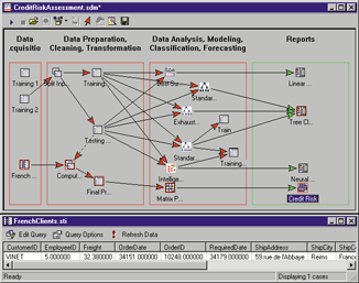
Data Preparation (in Data Mining)
Data preparation and cleaning is an often neglected but extremely important step
in the data mining process. The old saying "garbage-in-garbage-out" is
particularly applicable to the typical data mining projects where large data
sets collected via some automatic methods (e.g., via the Web) serve as the input
into the analyses. Often, the method by which the data where gathered was not
tightly controlled, and so the data may contain out-of-range values (e.g.,
Income: -100), impossible data combinations (e.g., Gender: Male, Pregnant: Yes),
and the like. Analyzing data that has not been carefully screened for such
problems can produce highly misleading results, in particular in
predictive data mining.
Data Reduction (for Data Mining)
The term Data Reduction in the context of data mining is usually applied to
projects where the goal is to aggregate or amalgamate the information contained
in large datasets into manageable (smaller) information nuggets. Data reduction
methods can include simple tabulation, aggregation (computing descriptive
statistics) or more sophisticated techniques like
clustering,
principal components analysis, etc.
See also predictive data mining, drill-down analysis.
Deployment
The concept of deployment in predictive data mining
refers to the application of a model for prediction or classification to new
data. After a satisfactory model or set of models has been identified (trained)
for a particular application, one usually wants to deploy those models so that
predictions or predicted classifications can quickly be obtained for new data.
For example, a credit card company may want to deploy a trained model or set of
models (e.g., neural networks, meta-learner) to quickly
identify transactions which have a high probability of being fraudulent.
Drill-Down Analysis
The concept of drill-down analysis applies to the area of data mining, to denote
the interactive exploration of data, in particular of large databases. The
process of drill-down analyses begins by considering some simple break-downs of
the data by a few variables of interest (e.g., Gender, geographic region, etc.).
Various statistics, tables, histograms, and other graphical summaries can be
computed for each group. Next one may want to "drill-down" to expose and further
analyze the data "underneath" one of the categorizations, for example, one might
want to further review the data for males from the mid-west. Again, various
statistical and graphical summaries can be computed for those cases only, which
might suggest further break-downs by other variables (e.g., income, age, etc.).
At the lowest ("bottom") level are the raw data: For example, you may want to
review the addresses of male customers from one region, for a certain income
group, etc., and to offer to those customers some particular services of
particular utility to that group.
Feature Selection
One of the preliminary stage in
predictive data mining, when the data set includes more variables than could
be included (or would be efficient to include) in the actual model building
phase (or even in initial exploratory operations), is to select predictors from
a large list of candidates. For example, when data are collected via automated
(computerized) methods, it is not uncommon that measurements are recorded for
thousands or hundreds of thousands (or more) of predictors. The standard
analytic methods for predictive data mining, such as
neural
network analyses,
classification and regression trees,
generalized linear models, or
general linear models become impractical when the number of predictors
exceed more than a few hundred variables.
Feature selection selects a subset of predictors from a large list of candidate predictors without assuming that the relationships between the predictors and the dependent or outcome variables of interest are linear, or even monotone. Therefore, this is used as a pre-processor for predictive data mining, to select manageable sets of predictors that are likely related to the dependent (outcome) variables of interest, for further analyses with any of the other methods for regression and classification.
Machine Learning
Machine learning, computational learning theory, and similar terms are often
used in the context of
Data Mining,
to denote the application of generic model-fitting or classification algorithms
for predictive data mining. Unlike traditional statistical
data analysis, which is usually concerned with the estimation of population
parameters by statistical inference, the emphasis in data mining (and machine
learning) is usually on the accuracy of prediction (predicted classification),
regardless of whether or not the "models" or techniques that are used to
generate the prediction is interpretable or open to simple explanation. Good
examples of this type of technique often applied to predictive
data mining are neural networks or meta-learning techniques
such as boosting, etc. These methods usually involve the
fitting of very complex "generic" models, that are not related to any reasoning
or theoretical understanding of underlying causal processes; instead, these
techniques can be shown to generate accurate predictions or classification in
crossvalidation samples.
Meta-Learning
The concept of meta-learning applies to the area of predictive
data mining, to combine the predictions from multiple models. It is
particularly useful when the types of models included in the project are very
different. In this context, this procedure is also referred to as
Stacking (Stacked Generalization).
Suppose your data mining project includes tree classifiers, such as C&RT and CHAID, linear discriminant analysis (e.g., see GDA), and Neural Networks. Each computes predicted classifications for a crossvalidation sample, from which overall goodness-of-fit statistics (e.g., misclassification rates) can be computed. Experience has shown that combining the predictions from multiple methods often yields more accurate predictions than can be derived from any one method (e.g., see Witten and Frank, 2000). The predictions from different classifiers can be used as input into a meta-learner, which will attempt to combine the predictions to create a final best predicted classification. So, for example, the predicted classifications from the tree classifiers, linear model, and the neural network classifier(s) can be used as input variables into a neural network meta-classifier, which will attempt to "learn" from the data how to combine the predictions from the different models to yield maximum classification accuracy.
One can apply meta-learners to the results from different meta-learners to create "meta-meta"-learners, and so on; however, in practice such exponential increase in the amount of data processing, in order to derive an accurate prediction, will yield less and less marginal utility.
Models for Data Mining
In the business environment, complex
data mining
projects may require the coordinate efforts of various experts, stakeholders, or
departments throughout an entire organization. In the data mining literature,
various "general frameworks" have been proposed to serve as blueprints for how
to organize the process of gathering data, analyzing data, disseminating
results, implementing results, and monitoring improvements.
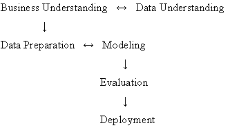
One such model, CRISP (Cross-Industry Standard Process for data mining) was proposed in the mid-1990s by a European consortium of companies to serve as a non-proprietary standard process model for data mining. This general approach postulates the following (perhaps not particularly controversial) general sequence of steps for data mining projects:
Another approach - the Six Sigma methodology - is a well-structured, data-driven methodology for eliminating defects, waste, or quality control problems of all kinds in manufacturing, service delivery, management, and other business activities. This model has recently become very popular (due to its successful implementations) in various American industries, and it appears to gain favor worldwide. It postulated a sequence of, so-called, DMAIC steps -

- that grew up from the manufacturing, quality improvement, and process control traditions and is particularly well suited to production environments (including "production of services," i.e., service industries).
Another framework of this kind (actually somewhat similar to Six Sigma) is the approach proposed by SAS Institute called SEMMA -

- which is focusing more on the technical activities typically involved in a data mining project.
All of these models are concerned with the process of how to integrate data mining methodology into an organization, how to "convert data into information," how to involve important stake-holders, and how to disseminate the information in a form that can easily be converted by stake-holders into resources for strategic decision making.
Some software tools for data mining are specifically designed and documented to fit into one of these specific frameworks.
��
Predictive Data Mining
The term Predictive Data Mining is usually applied to identify data mining
projects with the goal to identify a statistical or neural network model or set
of models that can be used to predict some response of interest. For example, a
credit card company may want to engage in predictive data mining, to derive a
(trained) model or set of models (e.g., neural networks,
meta-learner) that can quickly identify transactions which have a high
probability of being fraudulent. Other types of data mining projects may be more
exploratory in nature (e.g., to identify cluster or segments of customers), in
which case drill-down descriptive and exploratory methods
would be applied. Data reduction is another possible
objective for data mining (e.g., to aggregate or amalgamate the information in
very large data sets into useful and manageable chunks).
SEMMA
See Models for Data Mining.
Stacked Generalization
See Stacking.
Stacking (Stacked Generalization)
The concept of stacking (short for Stacked Generalization) applies to the area
of predictive data mining, to combine the predictions from
multiple models. It is particularly useful when the types of models included in
the project are very different.
Suppose your data mining project includes tree classifiers, such as C&RT or CHAID, linear discriminant analysis (e.g., see GDA), and Neural Networks. Each computes predicted classifications for a crossvalidation sample, from which overall goodness-of-fit statistics (e.g., misclassification rates) can be computed. Experience has shown that combining the predictions from multiple methods often yields more accurate predictions than can be derived from any one method (e.g., see Witten and Frank, 2000). In stacking, the predictions from different classifiers are used as input into a meta-learner, which attempts to combine the predictions to create a final best predicted classification. So, for example, the predicted classifications from the tree classifiers, linear model, and the neural network classifier(s) can be used as input variables into a neural network meta-classifier, which will attempt to "learn" from the data how to combine the predictions from the different models to yield maximum classification accuracy.
Other methods for combining the prediction from multiple models or methods (e.g., from multiple datasets used for learning) are Boosting and Bagging (Voting).
Text Mining
While Data
Mining is typically concerned with the detection of patterns in numeric
data, very often important (e.g., critical to business) information is stored in
the form of text. Unlike numeric data, text is often amorphous, and difficult to
deal with. Text mining generally consists of the analysis of (multiple) text
documents by extracting key phrases, concepts, etc. and the preparation of the
text processed in that manner for further analyses with numeric data mining
techniques (e.g., to determine co-occurrences of concepts, key phrases, names,
addresses, product names, etc.).
Suppose that (X1, X2, ..., Xn) is a random sample from the normal distribution with mean µ and standard deviation d. In this section, we will establish several special properties of the sample mean, the sample variance, and some other important statistics.
First recall that the sample mean is
M = (1 / n)![]() i
= 1, ..., n Xi.
i
= 1, ..., n Xi.
The distribution of the M follows easily from basic properties of independent normal variables:
![]() 1.
Show that M is normally distributed with mean µ and variance d2
/ n.
1.
Show that M is normally distributed with mean µ and variance d2
/ n.
![]() 2.
Show that Z = (M - µ) / (d / n1/2)
has the standard normal distribution.
2.
Show that Z = (M - µ) / (d / n1/2)
has the standard normal distribution.
The standard score Z will appear in several of the derivations below.
Recall that if µ is known, a natural estimator of the variance d2 is
W2 = (1 / n)![]() i
= 1, ..., n (Xi - µ)2.
i
= 1, ..., n (Xi - µ)2.
Although the assumption that µ is known is usually artificial, W2 is very easy to analyze and it will be used in some of the derivations below.
![]() 3.
Show that nW2 / d2 has the
chi-square distribution with n degrees of freedom.
3.
Show that nW2 / d2 has the
chi-square distribution with n degrees of freedom.
![]() 4.
Use the result of the previous exercise to show that
4.
Use the result of the previous exercise to show that
Recall that the sample variance is
S2 = [1 / (n -
1)]![]() i
= 1, ..., n (Xi - M)2.
i
= 1, ..., n (Xi - M)2.
The next series of exercises show that the sample mean M and the sample variance S2 are independent. First we will note a simple but interesting fact, that holds for a random sample from any distribution, not just the normal.
![]() 5.
Use basic
properties of covariance to show that for each i, M
and Xi - M are uncorrelated:
5.
Use basic
properties of covariance to show that for each i, M
and Xi - M are uncorrelated:
Our analysis hinges on the sample mean M and the vector of deviations from the sample mean:
Y = (X1 - M, X2 - M, ..., Xn - 1 - M).
![]() 6.
Show that
6.
Show that
Xn - M = -![]() i
= 1, ..., n - 1 (Xi - M).
i
= 1, ..., n - 1 (Xi - M).
and hence show that S2 can be written as a function of Y.
![]() 7.
Show that the M and the vector Y have a joint
multivariate normal distribution.
7.
Show that the M and the vector Y have a joint
multivariate normal distribution.
![]() 8.
Use the results of the previous exercises to show that M and the
vector Y are independent.
8.
Use the results of the previous exercises to show that M and the
vector Y are independent.
![]() 9.
Finally, show that M and S2 are independent.
9.
Finally, show that M and S2 are independent.
We can now determine the distribution of the sample variance S2.
![]() 10.
Show that nW2 / d2 = (n -
1)S2 / d2 + Z2
where W2 and Z are as given above.
10.
Show that nW2 / d2 = (n -
1)S2 / d2 + Z2
where W2 and Z are as given above.
Hint: In the sum on the left, add and subtract M,
and expand.
![]() 11.
Show that (n - 1) S2 / d2
has the chi-squared distribution with n - 1 degrees of freedom.
11.
Show that (n - 1) S2 / d2
has the chi-squared distribution with n - 1 degrees of freedom.
Hint: Use the result of the previous exercise,
independence, and moment generating functions.
![]() 12.
Use the result of the previous exercise to show that
12.
Use the result of the previous exercise to show that
Of course, these are special cases of the general results obtained earlier.
The next sequence of exercises will derive the distribution of
T = (M - µ) / (S / n1/2).
![]() 13.
Show that T = Z / [V / (n - 1)]1/2.
where Z is as above and where V = (n - 1)
S2 / d2.
13.
Show that T = Z / [V / (n - 1)]1/2.
where Z is as above and where V = (n - 1)
S2 / d2.
![]() 14.
Use previous results to show that T has the
t
distribution with n - 1 degrees of freedom.
14.
Use previous results to show that T has the
t
distribution with n - 1 degrees of freedom.
The random variable T plays a critical role in constructing interval estimates for µ and performing hypothesis tests for µ.